The above produces three distinct groups in three iterations. This is fine if it is known that there are three groups; in K-Means the number of clusters is an input parameter, but what if you don't know how many clusters there should be (which is one of the purposes of cluster analysis!)? One method is to try several different numbers of clusters and watch how a score of performance changes with the number of clusters. The score is usually measured by the sum of squared errors (SSE), which measures how far away points assigned to a cluster are from the centroid of the cluster. Usually, as the mumber of clusters increases the SSE will drop quickly. However, as the number gets beyond a certain value there will be a fall off in the amount by which it drops, see below.
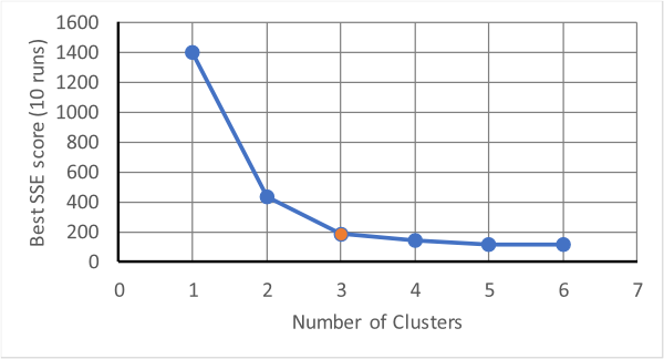 The point at which the drop-off changes is at three clusters in the above and this should
be tried as the minimum number with which to analyse the data. This method of determining the
number of clusters is known as the "elbow method" as it uses the "elbow" in the shape of the
data.
The point at which the drop-off changes is at three clusters in the above and this should
be tried as the minimum number with which to analyse the data. This method of determining the
number of clusters is known as the "elbow method" as it uses the "elbow" in the shape of the
data.
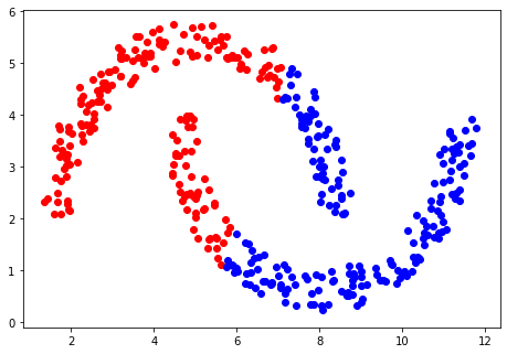
The method of K-Means separates data points linearly. This works well for the example above but when applied to a different set of data, the shortcoming of a linear separation is apparent.
 There are ways around this! It is possible to map each data point into a higher-dimensional
space, which, if the mapping is chosen carefully, will allow the desired separation. This
method is called the Kernel K-Means method, and requires a "Kernel" function to be defined
that represents not the data mapping but an inner product of the mapped data. Unfortunately, the best function to use depends on the data.
There are ways around this! It is possible to map each data point into a higher-dimensional
space, which, if the mapping is chosen carefully, will allow the desired separation. This
method is called the Kernel K-Means method, and requires a "Kernel" function to be defined
that represents not the data mapping but an inner product of the mapped data. Unfortunately, the best function to use depends on the data.
An alternative method is to look at the density of points and use this as a way of determining how they should be clustered. One density-based approach is known as DBSCAN (also available as a function in sklearn). This method looks at all the points and determines which are surrounded by a given minimum number of other points within a given radius. The points that are within this region are all classified as being the same and the method is then recursively applied to those points. Eventually, there will be no more points left within the region and the method starts a new class and moves on to the next unclassified point.
 At the end of the process most of the points will be assigned to a cluster,
with some that are at the edges of clusters, which can be assigned to the closest cluster available.
Others will be neither classified nor boundary points, and which will be discarded as being outliers. An
example classification using DBSCAN is shown below, and it can be seen that the data are correctly
separated, and, with the radius and minimum number of points chosen, two classes are defined.
At the end of the process most of the points will be assigned to a cluster,
with some that are at the edges of clusters, which can be assigned to the closest cluster available.
Others will be neither classified nor boundary points, and which will be discarded as being outliers. An
example classification using DBSCAN is shown below, and it can be seen that the data are correctly
separated, and, with the radius and minimum number of points chosen, two classes are defined.
 The DBSCAN method has the advantage that it automatically determines how many clusters there are
but the catch is the minimum number of points and the radius used for neighbour counting do have
to be specified. Again the choice is determined by the data.
The DBSCAN method has the advantage that it automatically determines how many clusters there are
but the catch is the minimum number of points and the radius used for neighbour counting do have
to be specified. Again the choice is determined by the data.
Note, these are not the only methods available!