What's the best?
Using optimisation methods
Optimisation is of great importance to many operations. It is the art of finding the best way to design or operate that achieves the most with the least effort or material use. By way of a simple example consider a humble cylindrical can used for food storage and preservation. An optimisation of the design might consider, for a given storage volume, what is the radius and height of the design that uses the least amount of metal? It is fairly easy to write an expression for how the surface area of metal used varies with the radius (the associated height is linked to the radius as the volume of the cylinder is a constant). The result can be found using a plot, or by calculus, and leads to the conclusion that food cans should be cyclinders with a height that is equal to their radius. A quick comparison with actual designs shows this isn't the case, as shown below.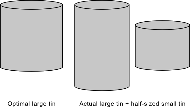
The reason why actual designs are different may arise from the fact that food producers often sell food cans in two sizes; a full-sized can, and a half-sized can, as shown above. This, then, becomes a problem in co-optimisation, which is very common. As a rule of thumb, optimising the individual components of a system does not generally lead to optimisation of the combined system.
For the co-optimisation of different sized cans some constraints should be considered. For ease of stacking the cans should have an equal radius, and the small can should be half the height of the large one. Again, it is reasonable easy to plot how the surfacte area of the combined production varies with product radius when the small cans are produced in the ratio n : 1 with the large ones, as shown below.
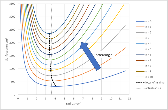
In this diagram, the thick dotted line connects all the radii for the best radius for the different production ratios n : 1. The thin dotted line shows a typical production radius. It is seen that if the production ratio of small : large is 2 : 1, the observed radius is approximately optimal. It is also apparent that the ratio can change from about 1 : 1 to about 6 : 1 or more and the radius remains very close to optimal.
Consider the case where cylinders of volume \(V_0\) and \(2V_0\) are co-manufactured in the ratio
of \(n:1\) subject to
- Both cylinders share a common radius, \(r\).
- The cylinder with volume \(V_0\) has a height \(h\) and the cylinder with volume \(2V_0\) has a height \(2h\).
The problem above can easily be solved using graphical or calculus methods. However, there are many cases where this is not the case because it is hard to write expressions that capture how an optimising variable changes with configuration, even though it is reasonably easy to write an expression for how optimal a configuration is. An example of this might be cutting shapes from a sheet of material; it's easy to measure how much wasted material there is, it's much harder to write a function that predicts exactly where each shape should go. In such cases other methods are required. Some of these use rules and perform systematic searches, others, such as genetic algorithms and simulated annealing start with random configurations and apply methods to guide how the cofiguration changes towards the optimal.
A gentic algorithm
A genetic algorithm is a method of optimisation that draws its inspiration from Darwinian Selection. The state of a problem is encoded in a set of "genes" in a population of "individuals". These "individuals" are ranked by how well they score against the desired measure and those that rank highest pass their genes on to the next generation by "mating" to produce offspring with a mixture of genetic characteristics of both parents. In the case of the can problem above, the genetic sequence of an individual is given by a set of digits that encode the radius of the can. For example, a radius of 3.23 is encoded by the gene sequence 323. The fitness of the individual is given by the can surface area this radius gives. Those with lower values are higher ranked and will mate more frequently. Mating to produce an offspring is achieved by constructing a new gene sequence where each gene has a random 50% chance of being derived from one or the other parent, as shown in the example below where a parent with radius 3.23 mates with another of radius 4.19 to produce an offspring with radius 3.19.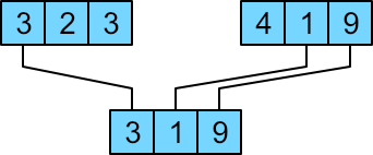
The above process is not enough however. The fitness criterion applied will eventually make the population genetically uniform and the process will stop. To allow for this another feature of Darwian Evolution is borrowed: the concept of random mutation. Under random mutation, each genetic element of the offspring is allowed to change randomly to another digit with probability \(P\). Note, \(P\) should be a reasonably small value otherwise the mutations will occur too frequently and the selection process will not work efficiently.
The example below demonstrates how a genetic algorithm with a population size of 20 can be used to determine the best radius for the can problem shown above (chosen, because we know what the answer should be). Once started, the population are ranked and used to produce offspring. These replace the parent population and the process repeats.